I really wish I'd been able to be at Milton Keynes on June 15th for Ira Greenberg's visit. I watched the proceedings a few days later via the webcast, and also tried out some of the sketches on Ira's website. Congratulations to those of you who volunteered to do presentations. They were really interesting. Well done!
Sunday, 28 June 2009
Friday, 8 May 2009
Chunk 67 finished
Tuesday, 5 May 2009
Chunk 67 - The final section
So now for some fun in creating some patterns using these functions. There are 5 examples shown here utilising a variety of techniques from wallpaper patterns using translation to geometric patterns using rotation and scaling and composite forms using a combination of all these functions.
1) Wallpaper patterns
Wallpaper patterns can use translation, reflection and rotation to create predictable pattern repeats of one or more motifs. A simple example is shown here that just uses translation. We've chosen to repeat the pattern along the horizontal and vertical axes but it would have been equally possible to repeat it along diagonals with the same effect.
The repeated motifs fit inside an 8 by 8 chequer board of squares. Alternate squares on each row will contain a diamond shaped motif and the positions of the motifs are staggered by one on each successive row. You might want to look at the finished display in figure (vii) at this point.
Here is the code for our Wallpaper program:
void setup(){

  size(300,300);

  background(152);

  noStroke();

  wallpaper();

}


void wallpaper(){

  float border = (min(height,width)- 160)/2;

  fill(204);  //pale grey

  rect(border,border,160,160);

  fill(102,255,204);


  for (int i= 0; i < 4; i++){

    translate(border, border+40*i);

    for (int j = 0; j <4; j++){

      quad(10,0,20,10, 10,20,0,10);

      translate(40,0);

    }

    resetMatrix();

    translate(border+20, border+40*i+20);


    for (int j = 0; j < 4; j++){

      quad(10,0,20,10, 10,20,0,10);

      translate(40,0);

    }

    resetMatrix();

  }

}
Let's examine the setup() function first:
void setup(){

  size(300,300);

  background(152);

  noStroke();

  wallpaper();

}
This sets the size of the display window, colours the background mid grey and turns off the pen using noStroke(). The work of the program is done by the function wallpaper().
The squares containing the motifs are going to be 20 by 20 pixels in size so we need 20 * 8 = 160 pixels in each direction. The size of the border needed is calculated using a function min() that you may not have seen before, which returns the smaller of its two arguments:
float border = (min(height,width)- 160)/2;
The next few lines lay out the light grey background to the motifs and set their fill colour :
  fill(204);

  rect(border,border,160,160);

  fill(102,255,204);
Nested for loops then creates the lines of motifs:
for (int i= 0; i < 4; i++){

    translate(border, border+40*i);

    for (int j = 0; j <4; j++){

      quad(10,0,20,10, 10,20,0,10);

      translate(40,0);

    }

    resetMatrix();


    translate(border+20, border+40*i+20);

    for (int j = 0; j < 4; j++){

      quad(10,0,20,10, 10,20,0,10);

      translate(40,0);

    }

    resetMatrix();

  }
The outer loop iterates through 4 pairs of rows. Within this, the coordinate axes are first translated to the top left square of the first of the pair of rows, then the motif is drawn for each column in turn. and translate is used to move 2 squares to the next column. Then the transformation matrix is reset. This is repeated for the second of the pair of rows with the motif offset by one column.
The finished result is shown in figure (vii) below.
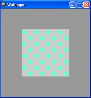
figure (vii)
2) Rotation used to build curved shapes
An example of this type of pattern is the sketch CollapsingBubbles which draws a spiral of overlapping circles. The program positions the first circle near the centre of the display window and gradually rotates the graphics context while moving the centre of the next circle nearer to the origin using the rotated axes. The code for the program is shown below.
void setup(){

  size(300,300);

  collapsingBubbles();

}


void collapsingBubbles(){

  float diameter = 20;

  float startX = (width / 2) - diameter;

  float startY = height / 2;

  float rotation = 0.1;

  float cumRotation = 0;

  while (cumRotation <50){

    ellipse(startX - cumRotation,

 startY - cumRotation, diameter, diameter);

    translate(width / 2 , height / 2);

    rotate(rotation);

    translate(- width / 2, - height / 2);

    cumRotation += rotation;

  }

}
The setup() function sets up the size of the window and calls the function collapsingBubbles(). This first of all sets the diameter of the bubbles and the x and y coordinates of the centre of the bounding box of the first bubble: startX and startY. Remember that the default mode for ellipses is ellipseMode(CENTER).
Two variables, rotation and cumRotation, are declared and initialised. rotation holds the angle in radians for each successive rotation. This is set to 0.1. cumRotation holds the cumulative angle of rotation.
A while loop then draws each successive circle using the value of diameter as the width and height of the bounding box:
while (cumRotation <10*TWO_PI){

    ellipse(startX - cumRotation,

 startY - cumRotation, diameter, diameter);

    translate(width / 2 , height / 2);

    rotate(rotation);

    translate(- width / 2, - height / 2);

    cumRotation += rotation;

}
The loop uses the variable cumRotation as an offset to the starting coordinates of the circle's centres. The graphics context is then rotated about the centre of the display screen by the angle in the variable rotation, ready for the next iteration, first translating the origin to the centre of the display window, the point (width/2, height/2), and resetting it back after the rotation by translating backwards by the same values along the rotated coordinate axes. The loop ends when cumulative angle of rotation, as incremented at the end of each iteration, is > 10 π.
Figure (viii) below shows the finished results.
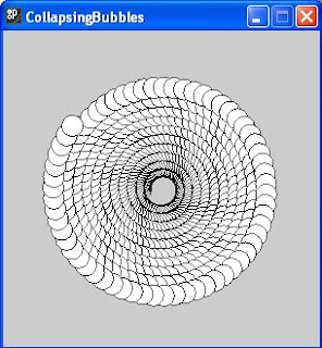
figure (viii)
3) Rotation using draw()
Another example illustrates the steps that are necessary to preserve the affine transformation matrix where iteration is achieved using the draw() function rather than a loop. Code for the program HouseofCards, which scatters squares using a little randomness, is shown below.
float rotation = 0.1;

float cumRotation=0;


void setup(){

  size(300,300);

  pushMatrix();

}


void draw(){

  popMatrix();

  translate(width/2+random(4),height/2+random(4));

  rotate(rotation);

  translate(-width/2-random(4),-height/2-random(4));

  rect(90+random(3),90-random(3),40,40);

  cumRotation+=rotation;

  pushMatrix();

}
The program is similar to that in the previous example which used
ellipses except that the coordinates of the bounding box, as well as the shift values used for the translations, have a slight random variation on each iteration. The default rectMode(CORNER) is implied here, which you'll remember is not the same default as for an ellipse.
The results of successive transformations are saved using pushMatrix() and popMatrix(), as was explained earlier. The variables rotation and cumRotation are also declared at the start of the program so that they are not reinitialised on every pass through the code of draw(), as they would be if they were local to a function. The results of one run allowing the draw function to execute until the cumulative rotation is around 40π radians is shown below in figure (ix).
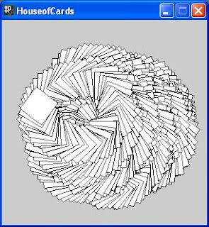
Figure (ix)
4) Kaleidoscopic effects of scaling and rotation
Kaleidoscopes use reflection to produce riots of colourful geometric patterns. However rotation and scaling can produce equally amazing patterns as is shown by the CascadingStars program. This displays a single triangle, successively rotated and scaled about the centre of the display window, each time using a different colour, chosen randomly from a small pallet:
void setup(){

  size(300,300);

  cascadingStars();

}


void cascadingStars(){

  int[] colArray= {0,153,204,255};

  for (int i =0; i< 100; i++){

    fill( colArray[int(random(3.9))], colArray[int(random(3.9))],

            colArray[int(random(3.9))]);

    triangle(40,40,width-10,height-80, height/2-20,width/2+20);

    scale(0.9);

    translate(width/2, height/2);

    rotate(i);

    translate(-width/2, -height/2);

  }

}
The setup() function sets the size of the output window, then calls the function cascadingStars().This first declares an array colArray which holds values which will be drawn from randomly as red green and blue colour values.
The function sets up a for loop which iterates round a number of times to display coloured triangles. On each pass, the function fill() is called to set the fill colour for the next triangle. The arguments are drawn randomly from colArray using:
colArray[int(random(3.9))]
random(3.9) returns a number between zero and 3.9 inclusive and int() rounds this to the integer below so that indices for colArray will be between 0 and 3.
The triangle is then drawn using the function triangle(). The arguments to the function are the x and y coordinates of each vertex and these were chosen arbitrarily. The graphics context is then scaled by a factor of 0.9 and rotated by 1 radian about the centre of the display window as in the CollapsingBubbles example above:
    scale(0.9);

    translate(width/2, height/2);

    rotate(i);

    translate(-width/2, -height/2);
One run of the program is shown in figure (x) below. A myriad of different colour combinations were produced on other runs.
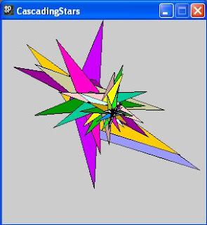
figure (x)
5) Solid geometric forms produced using scaling translation and rotation
Scaling can also be used to good effect in conjunction with translation to produce impressions of solid objects such as in figure (xi) below, where rotation has been used in addition to create the effect of a curved animal horn:
void setup(){

  size(300,300);

  antelopeHorn();

}


void antelopeHorn(){

  float i=0.01;

  float cumI=0;

  while (cumI <1.5){

    translate(width/2,height/2);

    rotate(-i);

    translate(-width/2,-height/2);

    scale(0.99);

    ellipse(280,280,30,30);

    cumI+=i;

  }

}
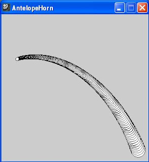
figure (xi)
We leave it as a task for the reader to work out how this example works.
Examples in this chunk have shown how translate(), scale() and rotate() can be used with the primitive 2D shapes: ellipse, rectangle, triangle and quadrilateral, created using Processing's ellipse(), rect(), triangle() and quad() functions. It's hoped that you'll want to experiment with sketches of your own using other shapes including arcs constructed using arc().
References
[1] Greenberg, Ira (2007) 'Shapes' Processing, Published: Berkeley California, Apress, Ch9 pp350-357.
[2] Cay S. Horstmann; Gary Cornell (2008 ) 'Advanced AWT>Coordinate Transformations' Core Java™ Volume II–Advanced Features, Eighth Edition. Published: Santa Clara, California, Sun Microsystems Inc. , Ch 7 pp552-556.
Sunday, 3 May 2009
Chunk 67 Sketch
I probably should stop playing with the sketch for chunk 67, SunsetBeach, and put the rest of the chunk up here for everyone to see. A quote from Strength to Love (Paul Gardener 1963) sums up its present state of flux better than I could have done: "A painting is never finished. It simply stops in an interesting place".
Here it is anyhow - comments welcome.
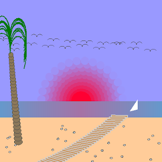
The quote was a recollection at http://musicthoughts.com/t/659
Friday, 1 May 2009
CHUNK 67 - the first 1300 words
TITLE Transformations
DESCRIPTION In this part of the book describe how shapes can be transformed.
OUTCOME Be able to use the transformation facilities in Processing to transform shapes previously introduced.
REFERENCE Greenberg 350--357
PROGRAM Develop a program that uses transformations of around 100-150 lines of code.
Processing has a number of functions which can be used to transform shapes. This chunk will describe how these can be used to draw any of the 2D primitive shapes introduced in chunk 66, but the same techniques will be used later on to transform more complex shapes such as those defined using OO classes as discussed in chunk 69. It's assumed that you have already read chunk 21 which discussed the basics of the coordinate system and how Processing uses this to display pixels on the screen.
The three functions that are needed for transforming shapes are:
translate(), scale() and rotate()
These don't merely take a shape and relocate or resize it, they alter the coordinate axes of the graphics context that will be used to display the shapes, so some understanding of how this works is necessary first of all.
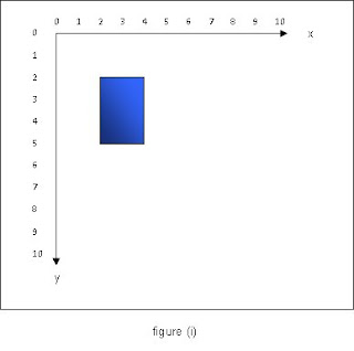
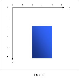
Figure (i) above shows a blue filled rectangle with width 2 and height 3 positioned with its top left hand corner at the point (2,2). Suppose xShift and yShift are the amounts the x and y axes respectively are to be translated by in the positive x and y directions. If the function:
translate(xShift, yShift)
is applied to the graphics context then the rectangle appears to be positioned on a different part of the screen. What is actually happening is that the coordinate system has changed and the origin has moved, so for example, if translate(2,3) is applied before drawing the rectangle, then the origin will move 2 units in the direction of the positive x axis and 3 units in the direction of the positive y axis, so that when the rectangle is drawn, its position will be that in figure (ii) below.
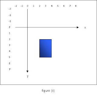
The rectangle will appear to be in a different place but the coordinates of its bounding box remain the same. It is of course quite possible to apply a translation which is large enough that shapes are no longer displayed on a visible part of the screen. This will become a problem once rotation is applied as will be explained later.
The effects of applying a scaling are similar. If xScaleFactor and yScaleFactor are the amounts by which the x and y axes are to be scaled, then applying the function:
scale(xScaleFactor, yScaleFactor)
to the graphics context will have the effect of making shapes drawn on it appear bigger or smaller, depending on the size of the scale factor. Figure (iii) below shows what happens when scale(2,2) is applied before drawing the rectangle. It appears to be twice its original width and height and be positioned further away from the origin, but in fact the coordinates of its bounding box have remained unchanged.
Processing has a number of constants built in that are useful when working with rotations. PI was used in an earlier chunk but the remainder of these may be new to you:
| Constant | Radians | (Degrees) |
|---|---|---|
| TWO_PI | 2π | (360°) |
| PI | π | (180°) |
| HALF_PI | π/2 | (90°) |
| QUARTER_PI | π/4 | (45°) |
Their values are in radians and they can be used as arguments, e.g.
rotate(QUARTER_PI)
The rotate() function rotates the graphics context clockwise through the number of radians given by its argument. You might imagine that this function would be similar in concept to translate() and scale(), however there is an added complication here in that the centre of rotation of the graphics context is the origin. This means that, for example, if you rotated the axes about π/2, then the entire sketch would be outside the visible area. To understand why this is so, look at what appears to happen to the grey rectangle when rotate(HALF_PI) is applied. Figure (iv) below shows that the coordinate axes rotate clockwise through 90°, so that its new position is that of the blue rectangle.
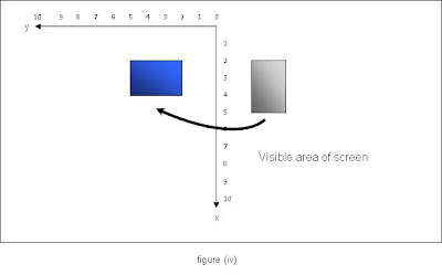
The visible portion of the screen is that to the right of the x axis. If the rectangle's location is as illustrated above, it won't be seen at all!
What is needed to rotate a shape around a different point, for example the centre of the screen, is first to translate the origin to the centre of the screen, then perform the rotation, and then translate the origin back again in the direction of the new axes by the same amounts as the original translation. Thus the following lines of code would rotate the graphics context through HALF_PI about the point (xShift, yShift):
      translate(xShift, yShift);
      rotate(HALF_PI);
      translate(-xShift, -yShift);
Rotation about the centre of the screen could be achieved by setting xShift to width/2 and yShift to height/2. Rotation about any other point can be achieved in the same way. Figure (v) below shows the effect of rotating the graphics context about the point (5,5) before drawing the same rectangle as before.
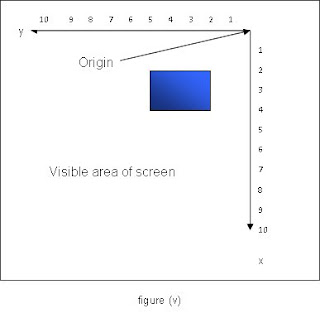
The coordinate axes are still rotated through 90°, but the origin has been translated first to the centre of the screen and then to the top right hand corner, so that the area bounded by the positive x and y axes is now visible.
The effects of the transformation functions are cumulative. That means that if you applied both scale() and translate() before drawing a shape then the coordinate axes would be scaled as well as the origin being translated. If you scaled them by 3 and then scaled them by 3 again, in both x and y directions, then the result would be to scale them by 3 * 3 = 9. A function resetMatrix() can be applied between transformations if this is not the intended effect. This changes the underlying affine transformation matrix back to its original settings. It's not necessary to consider the workings of this matrix in great detail here, but there's a reference [2] which explains the workings of the underlying Java AffineTransform class at the end of this chunk if you'd like to know more about how it works.
There is just one further consideration before we look at some examples of these functions in action. If the code to draw the shapes is placed in a draw() function, then on each iteration of the code within this, the affine transformation matrix will have been reset. This is equivalent to having performed resetMatrix() in each iteration of a loop. If you want to build up transformations cumulatively using draw(), then you will need a way to store the current transformation and restore it next time draw() is called. This is achieved using a matrix stack in Processing, as shown in figure (vi) below.
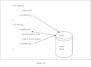
A call to popMatrix() at the start of the draw() function restores the affine transformation matrix by removing the top matrix from the stack and a call to pushMatrix() at the end of the function places the new affine transformation matrix at the top of the stack. A word of warning though; there has to be a matrix on the stack before you call popMatrix(), so setup() would also need a pushMatrix() call.