So now for some fun in creating some patterns using these functions. There are 5 examples shown here utilising a variety of techniques from wallpaper patterns using translation to geometric patterns using rotation and scaling and composite forms using a combination of all these functions.
1) Wallpaper patterns
Wallpaper patterns can use translation, reflection and rotation to create predictable pattern repeats of one or more motifs. A simple example is shown here that just uses translation. We've chosen to repeat the pattern along the horizontal and vertical axes but it would have been equally possible to repeat it along diagonals with the same effect.
The repeated motifs fit inside an 8 by 8 chequer board of squares. Alternate squares on each row will contain a diamond shaped motif and the positions of the motifs are staggered by one on each successive row. You might want to look at the finished display in figure (vii) at this point.
Here is the code for our Wallpaper program:
void setup(){

  size(300,300);

  background(152);

  noStroke();

  wallpaper();

}


void wallpaper(){

  float border = (min(height,width)- 160)/2;

  fill(204);  //pale grey

  rect(border,border,160,160);

  fill(102,255,204);


  for (int i= 0; i < 4; i++){

    translate(border, border+40*i);

    for (int j = 0; j <4; j++){

      quad(10,0,20,10, 10,20,0,10);

      translate(40,0);

    }

    resetMatrix();

    translate(border+20, border+40*i+20);


    for (int j = 0; j < 4; j++){

      quad(10,0,20,10, 10,20,0,10);

      translate(40,0);

    }

    resetMatrix();

  }

}
Let's examine the setup() function first:
void setup(){

  size(300,300);

  background(152);

  noStroke();

  wallpaper();

}
This sets the size of the display window, colours the background mid grey and turns
off the pen using noStroke(). The work of the program is done by the function wallpaper().
The squares containing the motifs are going to be 20 by 20 pixels in size so we need 20 * 8 = 160 pixels in each direction. The size of the border needed is calculated using a function min() that you may not have seen before, which returns the smaller of its two arguments:
float border = (min(height,width)- 160)/2;
The next few lines lay out the light grey background to the motifs and set their fill colour :
  fill(204);

  rect(border,border,160,160);

  fill(102,255,204);
Nested for loops then creates the lines of motifs:
for (int i= 0; i < 4; i++){

    translate(border, border+40*i);

    for (int j = 0; j <4; j++){

      quad(10,0,20,10, 10,20,0,10);

      translate(40,0);

    }

    resetMatrix();


    translate(border+20, border+40*i+20);

    for (int j = 0; j < 4; j++){

      quad(10,0,20,10, 10,20,0,10);

      translate(40,0);

    }

    resetMatrix();

  }
The outer loop iterates through 4 pairs of rows. Within this, the
coordinate axes are first translated to the top left square of the first of the pair of rows, then the motif is drawn for each column in turn. and translate is used to move 2 squares to the next column. Then the transformation matrix is reset. This is repeated for the second of the pair of rows with the motif offset by one column.
The finished result is shown in figure (vii) below.
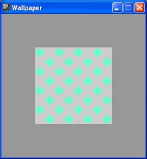
figure (vii)
2) Rotation used to build curved shapes
An example of this type of pattern is the sketch CollapsingBubbles which draws a spiral of overlapping circles. The program positions the first circle near the centre of the display window and gradually rotates the graphics context while moving the centre of the next circle nearer to the origin using the rotated axes. The code for the program is shown below.
void setup(){

  size(300,300);

  collapsingBubbles();

}


void collapsingBubbles(){

  float diameter = 20;

  float startX = (width / 2) - diameter;

  float startY = height / 2;

  float rotation = 0.1;

  float cumRotation = 0;

  while (cumRotation <50){

    ellipse(startX - cumRotation,

 startY - cumRotation, diameter, diameter);

    translate(width / 2 , height / 2);

    rotate(rotation);

    translate(- width / 2, - height / 2);

    cumRotation += rotation;

  }

}
The setup() function sets up the size of the window and calls the function
collapsingBubbles(). This first of all sets the diameter of the bubbles and the x and y coordinates of the centre of the bounding box of the first bubble: startX and startY. Remember that the default mode for ellipses is ellipseMode(CENTER).
Two variables, rotation and cumRotation, are declared and initialised. rotation holds the angle in radians for each successive rotation. This is set to 0.1. cumRotation holds the cumulative angle of rotation.
A while loop then draws each successive circle using the value of diameter as the width and height of the bounding box:
while (cumRotation <10*TWO_PI){

    ellipse(startX - cumRotation,

 startY - cumRotation, diameter, diameter);

    translate(width / 2 , height / 2);

    rotate(rotation);

    translate(- width / 2, - height / 2);

    cumRotation += rotation;

}
The loop uses the variable cumRotation as an offset to the starting coordinates
of the circle's centres. The graphics context is then rotated about the centre of the display screen by the angle in the variable rotation, ready for the next iteration, first translating the origin to the centre of the display window, the point (width/2, height/2), and resetting it back after the rotation by translating backwards by the same values along the rotated coordinate axes. The loop ends when cumulative angle of rotation, as incremented at the end of each iteration, is > 10 π.
Figure (viii) below shows the finished results.
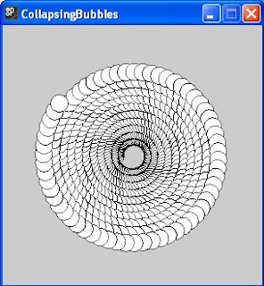
figure (viii)
3) Rotation using draw()
Another example illustrates the steps that are necessary to preserve the affine transformation matrix where iteration is achieved using the draw() function rather than a loop. Code for the program HouseofCards, which scatters squares using a little randomness, is shown below.
float rotation = 0.1;

float cumRotation=0;


void setup(){

  size(300,300);

  pushMatrix();

}


void draw(){

  popMatrix();

  translate(width/2+random(4),height/2+random(4));

  rotate(rotation);

  translate(-width/2-random(4),-height/2-random(4));

  rect(90+random(3),90-random(3),40,40);

  cumRotation+=rotation;

  pushMatrix();

}
The program is similar to that in the previous example which used
ellipses except that the coordinates of the bounding box, as well as the shift values used for the translations, have a slight random variation on each iteration. The default rectMode(CORNER) is implied here, which you'll remember is not the same default as for an ellipse.
The results of successive transformations are saved using pushMatrix() and popMatrix(), as was explained earlier. The variables rotation and cumRotation are also declared at the start of the program so that they are not reinitialised on every pass through the code of draw(), as they would be if they were local to a function. The results of one run allowing the draw function to execute until the cumulative rotation is around 40π radians is shown below in figure (ix).
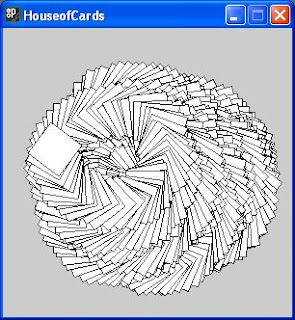
Figure (ix)
4) Kaleidoscopic effects of scaling and rotation
Kaleidoscopes use reflection to produce riots of colourful geometric patterns. However rotation and scaling can produce equally amazing patterns as is shown by the CascadingStars program. This displays a single triangle, successively rotated and scaled about the centre of the display window, each time using a different colour, chosen randomly from a small pallet:
void setup(){

  size(300,300);

  cascadingStars();

}


void cascadingStars(){

  int[] colArray= {0,153,204,255};

  for (int i =0; i< 100; i++){

    fill( colArray[int(random(3.9))], colArray[int(random(3.9))],

            colArray[int(random(3.9))]);

    triangle(40,40,width-10,height-80, height/2-20,width/2+20);

    scale(0.9);

    translate(width/2, height/2);

    rotate(i);

    translate(-width/2, -height/2);

  }

}
The setup() function sets the size of the output window, then calls the function
cascadingStars().This first declares an array colArray which holds values which will be drawn from randomly as red green and blue colour values.
The function sets up a for loop which iterates round a number of times to display coloured triangles. On each pass, the function fill() is called to set the fill colour for the next triangle. The arguments are drawn randomly from colArray using:
colArray[int(random(3.9))]
random(3.9) returns a number between zero and 3.9 inclusive
and int() rounds this to the integer below so that indices for colArray will be between 0 and 3.
The triangle is then drawn using the function triangle(). The arguments to the function are the x and y coordinates of each vertex and these were chosen arbitrarily. The graphics context is then scaled by a factor of 0.9 and rotated by 1 radian about the centre of the display window as in the CollapsingBubbles example above:
    scale(0.9);

    translate(width/2, height/2);

    rotate(i);

    translate(-width/2, -height/2);
One run of the program is shown in figure (x) below. A myriad of different colour combinations were produced on other runs.
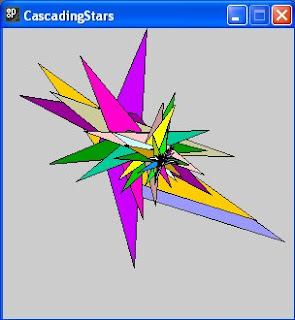
figure (x)
5) Solid geometric forms produced using scaling translation and rotation
Scaling can also be used to good effect in conjunction with translation to produce impressions of solid objects such as in figure (xi) below, where rotation has been used in addition to create the effect of a curved animal horn:
void setup(){

  size(300,300);

  antelopeHorn();

}


void antelopeHorn(){

  float i=0.01;

  float cumI=0;

  while (cumI <1.5){

    translate(width/2,height/2);

    rotate(-i);

    translate(-width/2,-height/2);

    scale(0.99);

    ellipse(280,280,30,30);

    cumI+=i;

  }

}
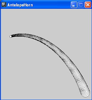
figure (xi)
We leave it as a task for the reader to work out how this example works.
Examples in this chunk have shown how translate(), scale() and rotate() can be used with the primitive 2D shapes: ellipse, rectangle, triangle and quadrilateral, created using Processing's ellipse(), rect(), triangle() and quad() functions. It's hoped that you'll want to experiment with sketches of your own using other shapes including arcs constructed using arc().
References
[1] Greenberg, Ira (2007) 'Shapes' Processing, Published: Berkeley California, Apress, Ch9 pp350-357.
[2] Cay S. Horstmann; Gary Cornell (2008 ) 'Advanced AWT>Coordinate Transformations' Core Java™ Volume II–Advanced Features, Eighth Edition. Published: Santa Clara, California, Sun Microsystems Inc. , Ch 7 pp552-556.


